Overview and structure
Apercal pipeline modules
The Apertif calibration pipeline Apercal is a combination of different modules, which are usually executed one after another. An overview of the whole reduction pipeline is given in Figure 1. Each rectangular box represents a single module. The grey boxes encapsulate the astronomical software packages used within the individual modules. Arrows illustrate the data and workflow within the pipeline. The dashed arrows and lines are routines which are currently in development.
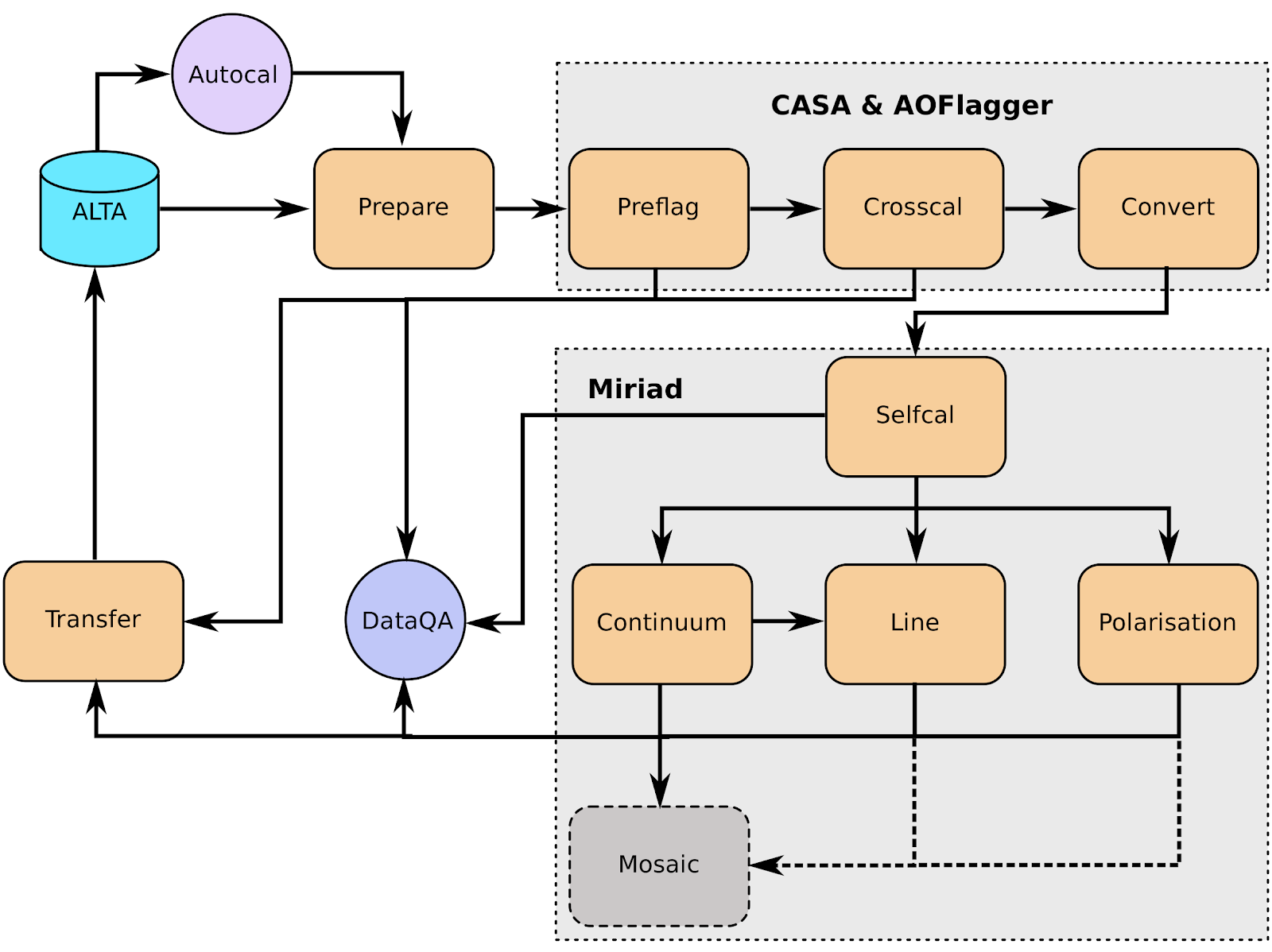
Figure 1.
At the top level, the role of each module is:
- AUTOCAL: The automated pipeline trigger, detecting new observations appearing in ALTA and starting a new pipeline call
- PREPARE: Sets up the directory structure used by Apercal and retrieves data from ALTA into this structure.
- PREFLAG: Flags the data
- CROSSCAL: Solves for and applies the cross-calibration solutions
- CONVERT: Converts the data from MS to miriad internal format
- SELFCAL: Derives and applies phase and (optional) amplitude gain solutions from the target dataset
- CONTINUUM: Produces continuum mfs images
- LINE: Produces dirty line cubes and corresponding dirty beam cubes
- POLARISATION: Produces Stokes V mfs images and Stokes Q & U cubes
- MOSAIC: In progress, produces mosaics of an observation and (eventually) between observations
- TRANSFER: Writes self-calibrated uv data to UVFITS format for archiving
In the following, we give more details on each of the individual modules.
When a new observation is uploaded to the Apertif Long Term Archive (ALTA), AUTOCAL automatically retrieves information about the target, flux and polarisation calibrator and triggers the start of the pipeline. Operating as a cron job, AUTOCAL first identifies a given observation as a target and then searches the Apertif Task DataBase (ATDB) for calibrators before and after.
Once AUTOCAL has successfully identified a target and the accompanying polarisation/flux calibrators, it sends all necessary information to Apercal, so that the pipeline can begin downloading the relevant data from ALTA. In addition to triggering the pipeline, AUTOCAL also triggers the automatic quality assessment (QA) pipeline, which inspects the raw data, calibration solutions and images, and ingests the processed data products back to ALTA, with associated notifications for each stage.
Apercal defines a directory structure for processing where each module uses its own subdirectory to access data and save outputs. All of the following modules (except CONVERT) use a single subdirectory, so that individual steps can easily be deleted and restarted. The naming of the directories can be adjusted to the needs of the users with keywords in the configuration file.
The main tasks of the PREPARE module are the setup of the directory structure and the download of the data. Once the module is executed given an input target and calibrator datasets, it checks the availability of the data on the local disc. In case data is not locally available, the module checks the availability on ALTA via an irods framework. If successful, a python routine is used to download the data to the local disc and to place it in the appropriate position of the directory structure. After a dataset has been successfully copied from ALTA or located on disc, the correctness of the file is checked via a checksum.
A minimum of a target dataset and a flux calibrator need to be present for this step to be successful. This condition ensures that, if no flux calibrator is available, the execution of the pipeline is stopped. On the other hand, the pipeline will continue when a polarised calibrator is not available. In this case, the polarisation calibration within the CROSSCAL module is omitted and no polarisation imaging is performed. We want to note that for pipeline runs using the automatic trigger via AUTOCAL a missing polarised calibrator is diagnosed as a failed observation and stops the pipeline.
The PREFLAG module handles all pre-calibration flagging of the data. It can be separated into three different operations: The flagging of data with issues known a priori, additional manual flagging, and automatic flagging routines to identify and mitigate spurious radio frequency interference (RFI). The first two operations use the drive-casa python wrapper to parse commands to CASA while the last one uses the AOFlagger routines.
The subroutines for a priori known issues cover three distinct operations: First the data is checked for shadowing effects, where the aperture of one dish is blocked by another. The next step is a mitigation of the effect of the steep bandpass edges of the individual subbands of the Apertif system. The first two and last channel of each 64 channel subband is flagged.
Subroutines for the manual flagging step encompass the removal of auto correlations, entire antennas, specific cross-correlations, individual baselines, channel and/or time ranges. Any flagging commands not covered by the standard commands can be parsed to a file using the standard CASA-syntax. All manual flags are supposed to be used either when known elements within the Apertif system are not working or a user identifies additional issues during calibration of the data. The data ranges to flag for the above mentioned subroutines are specified in the configuration file.
The last step of the module uses the AOFlagger (Offringa+ 2012) routines to automatically identify and flag any unknown and previously not flagged RFI in the calibrator and target datasets. A custom flagging strategy was designed which suits both, short calibrator and long target field observations.
During the cross calibration step, an astronomical point-like known reference source (a calibrator) is used to derive the calibration solutions, which are then transferred to an unknown target field.
The current calibration strategy encompasses a short flux and polarisation calibrator observation in the centre of each individual beam before or after a target field observation has been executed.
The cross-calibration step solves for the bandpass, gain, delay and polarisation leakage solutions of the flux calibrator. While the flux calibrator is unpolarised the cross-hand delay and polarisation angle solutions are derived from the polarised calibrator using the standard CASA routines. In case a polarisation calibrator has not been successfully observed or its dataset has not passed the PREFLAG module, polarisation leakage, polarisation angle and cross-hand delay solutions are not determined. Bandpass, polarisation leakage and polarisation angle solutions are derived on a per-channel basis to mitigate any effects within the observed bandwidth. For the unpolarised calibrators the flux density scale from Perley & Butler 2017 is used while for the additionally needed information for the polarised calibrators, such as the polarisation angle, degree of polarisation and Rotation Measure, Perley & Butler 2013 is used.
Calibrator data are automatically checked for problematic dish-beam combinations. Problems here arise from individual receiver elements in the PAF, which are malfunctioning due to broken connectors, cables or electronics. These problematic beams are spotted most easily in the auto-correlation data. Currently, this is done by checking the autocorrelations of the flux calibrator after a first cross-calibration for each dish/beam combination. The currently implemented metric checks that not more than 50% of the auto-correlation data show amplitudes of more than 1500 K, which is the value, derived from our experiences, where significant artefacts in the images become apparent. In addition the bandpass phase solutions of the flux calibrator are investigated after calibration for a standard deviation higher than 15°. If one of the above mentioned criteria applies to a dish-beam combination, the specified data is marked and flagged automatically. The flags are then applied to the target and polarisation calibrator data. The criteria determining the outcome of these metrics are dependent on the quality of the input data, so that the whole cross-calibration is performed in an iterative way. A maximum of four crosscal iterations are allowed after which the CROSSCAL module gives a final result. The pipeline is stopped for beams not passing this stage. If a beam passes the checks, all available calibrator solutions are applied to the target field dataset. Any further processing of the calibrator datasets stops here and the following modules only focus on the target data.
Since MIRIAD is not able to access the Measurement Set (MS)-format native to CASA, we need to convert the file format before doing any further reduction. Unfortunately a task for a direct conversion from MS to MIRIAD format is not available, so that we have to first convert to the UV-FITS standard and from there to MIRIAD. For this purpose we use the CASA task exportuvfits followed by the MIRIAD routine fits.
Self-calibration is a standard procedure in radio interferometric data reduction to enhance the dynamic range of images. Small changes in the processing of the signals in the receiver electronics (e.g. temperature changes) and ionospheric and tropospheric variations of the Earth’s atmosphere cause dampening of the received amplitudes and small delay variations, respectively, over the time of the target observations. These usually slowly changing variations cannot be compensated by the bracketing calibrator observations and therefore need self-calibration.
The task of the SELFCAL module is to solve for the antenna and feed time based variations of the target data within a self-regulating algorithm using the self-calibration technique. To guarantee the stability of the self-calibration process and the processing within a reasonable time frame, several preliminary steps are executed within SELFCAL before the actual self-calibration starts.
First, the target data is averaged down in frequency by a factor of 64 over the 64 channels of each subband resulting in a frequency resolution of 0.78 MHz to accelerate the self-calibration. We do not expect any strong amplitude or phase variations within this frequency span. It is important to note that this frequency averaged dataset is only used for continuum and polarisation imaging in later stages of the pipeline and any HI-line imaging is performed on a dataset with the original resolution where the derived self-calibration gains are interpolated and applied.
In order to mitigate any influence of strong HI-line emission or residual RFI on the self-calibration solutions we generate an image cube out of the averaged data. For each image in the cube its standard deviation is measured. An outlier detection algorithm is used to locate the channels affected by either above mentioned reasons and flag them in the averaged dataset. As above, these flags are only used for the continuum and polarisation imaging later in the pipeline and not for HI-line imaging.
The performance of the self-calibration is often strongly dependent on the first image passed to the solver. In order to start the self-calibration with an image of an optimal initial quality, we use the information provided by radio continuum surveys at the same wavelength. For this purpose we first query the catalogue of the Faint Images of the Radio Sky at Twenty-Centimeters (FIRST) Survey.
Since this survey does not cover the whole Apertif survey footprint information for fields outside of the FIRST footprint are collected from the Northern Very Large Array Sky Survey (NVSS). A fractional bandwidth of ~20% is used for observations, so that we need to account for the spectral index and primary beam variations over frequency. For acquiring a spectral index for the sources in our skymodel we query the Westerbork Northern Sky Survey (WENSS) catalogue and cross-match. Since WENSS has inferior resolution compared to the other two surveys, we account for multiple source matches by summing the fluxes of the individual components to derive the spectral index and assign the same value to all for them. We then account for the primary beam response of the Apertif system by using the primary beam model of the WSRT as an approximation. The final skymodel is then generated by directly fourier transforming the catalogue source fluxes and positions into the (u,v)-domain with the MIRIAD task uvmodel. This ensures that all our images are aligned to the same common reference frame given by the above mentioned surveys. In addition the resolution of this parametric skymodel is not limited by the pixel raster of the images, but rather the fitted position of the sources. The solution interval for this parametric calibration is usually on the order of several minutes, which is set in the config file.
The next step involves the actual self-calibration iterations. Each iteration consists of inverting the (u,v)-data using the MIRIAD task invert followed by an automatic masking routine involving the source finder PyBDSF to limit the CLEAN algorithm to islands of real emission. All self-calibration and imaging is performed on the total intensity Stokes I parameter. Image deconvolution is executed using the multi frequency CLEAN-algorithm implemented into the MIRIAD task mfclean, which uses a first order polynomial to derive the spectral index of the sources within the imaged bandwidth. After cleaning, restored and residual images are created using the task restor. The CLEAN model generated during the cleaning process is then used to derive new calibration solutions.
The CLEAN algorithm only performs perfectly for images which only consist of point-sources and do not show any calibration artefacts. Due to these circumstances and the fact that CLEAN is an iterative non-linear process, which can diverge, adaptive thresholds need to be set and constant quality assurance performed. For each cleaning process within a self-calibration cycle three different thresholds for generating masks are calculated: the theoretical noise threshold Ttn, the noise threshold Tnand the dynamic range threshold Tdr.
The theoretical noise T is determined by calculating the standard deviation from images generated in circular polarisation (Stokes V). Astronomical circular polarised sources are very rare on the sky and if present only at very low flux levels. Residual RFI on the other hand is often circular polarised and raises the noise levels of these images. The noise statistics of these images are therefore well representing the actual quality of the data and the theoretically reachable noise of the final images. Ttn is given in units of Jy and defined as
Ttn = T * nσ
where nσ is the confidence interval for regarding islands of emission as real. This is usually set to nσ=5. If at any during a CLEAN-cycle this limit is reached, the current cycle is finished and the self-calibration stops.
In order to guarantee a smooth convergence of the self-calibration skymodel the two additional thresholds Tdr and Tn set limits for the maximum dynamic range achievable in an image without reconstruction and the adaptation to image artefacts, respectively. The dynamic range threshold within a cycle is defined by the number of the current major cycle m, the initial dynamic range DRi and a factor defining how fast the threshold should increase DR0 such as
Tdr = Imax / (DRi * DR0m)
where Imax is the maximum pixel value in the residual image of the previous cycle. The parameter DRi is dependent on the level of the first major sidelobe in the dirty beam. The ratio between the maximum and this value gives the maximum dynamic range by which an image can be cleaned before another cycle of image reconstruction needs to be performed.
The adaption of the threshold for stopping each individual run of the CLEAN algorithm Tn is given by
Tn = Imax / ( (c0 + n*c0) (m+1) )
where n is the number of minor cycles and c0 handling how aggressive the cycles are performed. For each individual run of mfclean all three thresholds are calculated and the maximum set as a limit for the generation of masks in PyBDSF. Then cleaning is performed within this mask down to a level of the mask level divided by the parameter c1, which is usually set to c1=5.
The length of the solution interval s for each self-calibration cycle is determined by
s = ( t / ns) / m
where t is the total observation time, m again the iteration of the current major cycle and
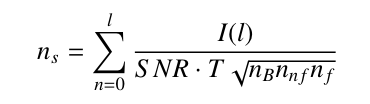
where l is the number of clean components, I the flux of each individual clean component, SNR the needed signal-to-noise ratio, T the theoretical noise, nB the number of baselines, nnf the number of solution intervals over frequency and nf the number of polarisations to solve for. SNR is set to 3 for phase-only calibration and to 10 for combined amplitude and phase calibration. These arithmetics ensure that solution intervals decrease during the self-calibration process consecutively while still containing enough signal-to-noise for a proper calibration.
The SELFCAL module first performs up to a given maximum number of iterations of phase-only self-calibration. Then it decides on the amount of flux and therefore the available SNR if and with which solution interval combined amplitude and phase self-calibration is executed. If at any point during the process the theoretical noise limit is reached, SELFCAL performs only one last iteration of self-calibration.
To improve the stability of the pipeline and the quality of the calibration solutions several metrics for quality assurance were implemented. At the beginning of each cycle, a multi-frequency image of circular polarisation (Stokes V) is generated. Since the circular polarised sky is essentially empty any sources in such an image would hint to severe calibration problems. Therefore, the image statistics can be analysed for following a normal distribution resembling Gaussian noise. This was implemented using the skewness and kurtosis of the distribution. If these values exceed a certain number given in the config-file, the self-calibration is aborted.
During and after each imaging and cleaning cycle the dirty image, the cleaning mask, the clean component model image and the restored images are checked for any obvious problems resulting from a divergence of the calibration routines. The maximum value in dirty images of total intensity should always exceed the minimum. In addition, no Not a Number (NaN)-values are expected in the image. Both conditions are checked when starting a cleaning where new solutions were derived and applied to the data and a new dirty image is generated. Masks are checked every time for containing any CLEAN components at all. The clean component image is checked for clean components with unrealistically strong negative or positive fluxes. The restored image is again checked for containing no NaN-values and for strong positive or negative values. The final residual image should mostly consist of noise and is therefore checked for gaussianity.
A combined amplitude and phase calibration (A&P) is not as stable as a phase-only calibration due to the increased degrees of freedom, so that this step can easily worsen the image quality due to diverging calibration solutions. Therefore, in addition to the quality assurance process described above, we added an additional metric to check the quality of the A&P calibration compared to the phase-only one. After the A&P calibration we generate another dirty image and compare the image statistics independently, namely its maximum, minimum and standard deviation with the dirty image of the last phase-only self-calibration cycle. If the ratio of one of those values exceeds a limit given in the config-file the A&P calibration is assessed as failed and any following module will use the last successful phase-only self-calibration solutions. Calibration solutions are applied in the subsequent modules before any further imaging is performed.
The CONTINUUM module performs two different tasks to generate final deep continuum Stokes I images. First it generates a deep multi-frequency image using the mfclean task in MIRIAD and secondly several individual images spanning narrower frequency ranges over the full bandwidth using the task clean are produced. The purpose of this is to generate an as deep as possible total intensity image with the maximum possible resolution (given by the highest frequency) and in addition derive reliable spectral indices and curvatures for as many sources as possible. In fact multi-frequency cleaning generates these images already, but their values are only reliable in cases of high signal-to-noise ratios. For both imaging steps we use a uniform weighting to acquire the maximum possible resolution on the order of 12’’. Images usually have a size of 3073×3073 pixels with a pixel size of 4 arcseconds, which allows the imaging and cleaning of any sources up to the first sidelobe level of the primary beam response in order to minimise artefacts.
Cleaning and masking iterations are in both cases continued until the theoretical noise limit has been reached. Masking and validation of all continuum images is performed in the same way as described for the SELFCAL module.
The LINE module first applies the derived self-calibration solutions to the non-averaged data. This is performed using the MIRIAD task gpcopy. It automatically takes care of the different frequency resolution of the two datasets by interpolation.
The HI-line imaging is the most computing intensive task in the Apertif data reduction, so that several endeavours have been undertaken to optimise its performance. For a better handling of the data and the image cubes imaging is performed by generating eight individual cubes over the 300 MHz of bandwidth with a small amount of overlap in frequency. The overlap is necessary to avoid splitting the detected line emission of individual objects between two adjacent image cubes. In order to improve sensitivity and save processing time and disc space, data between 1130 MHz and 1416 MHz are averaged in frequency by binning three channels together. The data at the highest frequencies which features the Galactic neutral hydrogen and small galaxies in the nearby Universe retains its full spectral resolution of 12.2 kHz.
In order to generate image cubes containing only HI-line emission the continuum has to be subtracted. Several different approaches are possible here: the fitting of baselines to the amplitude of the data followed by subtraction, the subtraction of constant fluxes over frequency in the image domain and the direct subtraction of a continuum clean component model from the (u,v)-data. The best performance in terms of time consumption was achieved with the latter method, so that we decided to use this in Apercal. For this subtraction the final clean model of the CONTINUUM module is used.
Finally the actual images are produced. MIRIAD does not account for the position dependence of sources situated outside of the pointing centre for large fractional bandwidth, if executed in line imaging mode. Therefore, we have to generate an image for each individual frequency and combine the final images into a cube. Since imaging of individual channels is very computing intensive, but also the imaging process for each individual channel is independent from another we optimised this step by implementing an OpenMP support with the python pymp library1.
1https://github.com/classner/pymp
Polarisation imaging is performed in Stokes Q, U and V. Q and U fluxes from astronomical sources exhibit a sinusoidal dependence of the square of the observed wavelength. In addition, Stokes Q, U and V fluxes can have negative values in contrast to Stokes I, which needs to be positive in all cases. These effects would lead to bandwidth depolarisation in case of multi-frequency imaging of Stokes Q and U over our full 300 MHz bandwidth. Therefore, we image Stokes Q and U as cubes, using the same method as described for the LINE module, where one image is generated for a bandwidth of 6.25 MHz. This mitigates the effect of bandwidth depolarisation for most astronomical sources. In addition, this method allows the usage of the Rotation Measure Synthesis technique in post-processing, so that the linear polarisation properties of the detected sources can be analysed in more detail than with the standard methods, which suffers from bandwidth depolarisation effects. Typical reachable Faraday Depth are still on the oder of several thousands, so that the polarised emission of nearly all astronomical sources is still recoverable with these specifications. Spatial resolution of the Stokes Q and U cubes is slightly lower (on the order of 15 arcseconds) in comparison to the continuum images.
Stokes V is representing the circular polarisation, which does not show any sinusoidal behaviour. Due to this fact and since the circular polarised sky is very faint, we perform a multi-frequency synthesis for imaging Stokes V. This also allows to maximise the sensitivity of the produced images to detect possible circular polarised sources.
For all polarisation images cleaning is performed using the final mask generated by the multi-frequency imaging part of the CONTINUUM module. Since polarisation images usually only show very faint emission, the clean threshold is set by the standard deviation of the pixels in the image. This accounts, especially for the Stokes Q and U images, for the variations of the noise over the imaged bandwidth. For cleaning Stokes Q and U we used the MIRIAD task clean and for Stokes V mfclean.
Currently we are not producing mosaics of the calibrated data during Apercal runs for the data release, but for reasons of completeness we explain the currently available mosaicking routines in the following. The mosaicking routines are independently implemented in order to address features specific to Apertif, namely varying primary beam responses for the different beams (see “Overview of primary beam shapes for Apertif“) and the ability to include correlated noise.
Once all data of an observation have been processed through the CONTINUUM, LINE and POLARISATION modules, the MOSAIC module is executed to generate a combined image of all beams of one observation taking into account the response of each compound beam. Images are regridded to a common grid centred on the central beam of the observation and then corrected for the Apertif compound beam response. The compound beam response has been characterised using drift scans of a strong astronomical source over the whole field of view of the Apertif Phased Array Feed (see Compound beam shape section). The different beams of one observation have slightly varying synthesised beam sizes due to different flagging of the data, so that all input images are convolved to the largest common beam.
The combination of the input images then follows an inverse square weighting based on the compound beam response and the background noise of the individual images. The background noise is estimated using the MIRIAD task sigest, which minimises the contribution of sources for the determination of the noise level.
Since all data of one observation has been taken using the same electronics, a correlation between the noise of different beams exists, which raises the noise level of the final mosaic. An option for including this correlation matrix during mosacking is implemented and will be used once the coefficients have been measured. First tests showed a minor change of the noise levels between correlated and uncorrelated data of adjacent beams of ~2%.
The MOSAIC module is currently only producing continuum mosaics using the central frequency of the observational setup for correcting the primary beam response. Additional features in the future include the implementation of the frequency and long-term time dependence of the beam pattern and the combination of images of different observations. The current implementation takes approximately an hour for generating a continuum mosaic. Future improvements will include enhancements to the speed of the module, which will then allow us to generate polarisation and line mosaics within an acceptable amount of time.
This module converts the self-calibrated MIRIAD data to more standard UVFITS format. Similar to LINE it applies the phase and, if available, amplitude self-calibration solutions to the non-averaged cross-calibrated data automatically before conversion. The calibrated visibility data, along with calibration tables and fits images/cubes, are then ready for archive ingest.
SEE ALSO: