LOFAR stations are complete, self-contained radio telescopes. Every station is equipped with its own correlator. The stations can operate in 5 different frequency ranges: 10–80, 30–80, 110–190, 170–230, and 210–250 MHz. The first two modes use the LBA antennae, the others the HBA. The antenna voltages can be sampled at either 160 MHz or 200 MHz. The station correlator has the following operating modes:

• Computing dynamic spectra over the full frequency range of a certain

filter/clock combination for all antennae;

• Computing a full array correlation matrix in one sub band.

These data products are extremely useful for diagnosing problems in an observation.

Participants are assumed to have

• basic Python programming knowledge;
• an idea about the signal path within a station;
• a basic understanding of radio interferometry.

The goal of this exercise is to familiarize yourself with the full array correlation matrices (ACM) from the station correlator, as well as the diurnal total power variations in the system. After this exercise you should be able to

• inspect and verify array correlation matrices;
• recognize an X or Y dipole orientation from the total power curves;
• produce visibility curves as a function of time for a variety of

baseline lengths;

• tell us which signal paths should be repaired;
• tell us which antenna was wired the wrong way around.

• `lofarstation.py` is the Python software for reading

and plotting the station correlator data;

• `lofarstation.html` is a nicely rendered version of

`lofarstation.py`;

• `cs010.py` contains the positions of the LBA dipoles on CS010;
• `array-correlation-matrices` contains the subdirectories with the

array correlation matrices for this exercise;

• `Exercise-02B.txt` is the plain text version of this instruction;
• `Exercise-02B.html` is the HTML version of this instruction.

The first thing to do is changing to the exercise directory and starting the IPython shell:

$ cd /data/lofarschool/users/station/Exercise-02B-station/
$ ipython -pylab lofarstation.py

the screen should now look something like this:

Python 2.5.1 (r251:54863, Jul 31 2008, 23:17:43) 
Type "copyright", "credits" or "license" for more information.
 
IPython 0.8.1 -- An enhanced Interactive Python.
?       -> Introduction to IPython's features.
%magic  -> Information about IPython's 'magic' % functions.
help    -> Python's own help system.
object? -> Details about 'object'. ?object also works, ?? prints more.
 
  Welcome to pylab, a matplotlib-based Python environment.
  For more information, type 'help(pylab)'.
 
In [1]: 

You may want to review the contents of lofarstation.py while doing this exercise.

The command `station_correlator_directories()` lists the directories that contain the dynamic spectra:

In [1]: station_correlator_directories()
Out[1]: 
[u'array-correlation-matrices/20081204-freq-scan',
 u'array-correlation-matrices/20081204-freq-scan-wg',
 u'array-correlation-matrices/20090202-school-acm-sb305-rcumode4']

The datasets were all recorded in LBA mode with the clock at 200 MHz. The top two datasets used RCU mode 3 and the last one RCU mode 4. The top two datasets contain frequency sweeps with the station correlator. Each directory contains 512 array correlation matrices recorded with 1 second integration time. The first ACM is recorded in sub band 0, the next in 1, and the last one in sub band 511. The first directory contains correlations of the antenna signals. The second one consists of cross correlations of waveform generator signals. These waveform generator signals are very strong and can be controlled by the observers. The most recent dataset is a 24 hour observation in sub band 305 with 60 seconds integration per time step.

The contents of a directory can be viewed with e.g.

In [2]: full_path_listdir(station_correlator_directories()[-1])
Out[2]: [u'array-correlation-matrices/2009....-rcumode4/20090202_090356_xst.dat']

The data file name consists of the UTC date and time of the start of the first integration and the letters `_xst_`, which indicate that the file contains cross correlations (array correlation matrices).

The `data_files()` function returns a list of all `.dat` files in a directory:

In [3]: files = data_files(u'array-correlation-matrices/20081204-freq-scan-wg')
In [4]: len(files)
Out[4]: 512
In [5]: files[0:3]
Out[5]:
[u'array-correlation-matrices/20081204-freq-scan-wg/20081204_090456_xst.dat',
 u'array-correlation-matrices/20081204-freq-scan-wg/20081204_090502_xst.dat',
 u'array-correlation-matrices/20081204-freq-scan-wg/20081204_090508_xst.dat']

The function `timeslots_in_acm_cube()` counts how many integrations are stored in a file.

In [6]: timeslots_in_acm_cube(data_files('array-correlation-matrices/20081204-freq-scan/')[256])
Out[6]: 1L
In [7]: timeslots_in_acm_cube('array-correlation-matrices/20090202-school-acm-sb305-rcumode4/20090202_090356_xst.dat')
Out[7]: 1432L

A file containing a single ACM can be read with the `read_acm()` function. If a file contains multiple ACMs, use the `read_acm_cube()` function. We are now going to read a couple of different array correlation matrices, which are all recorded in subband 305. The central frequency of this subband is

In [8]: subband_frequencies_mhz()[305]
Out[8]: 59.5703125

We assign variable names to the ACMs in order to make handling them a bit easier.

In [9]: acm_sky=read_acm(
   data_files('array-correlation-matrices/20081204-freq-scan/')[305])
In [10]: acm_wg=read_acm(
   data_files('array-correlation-matrices/20081204-freq-scan-wg/')[305])
In [11]: acmcube=read_acm_cube(
   'array-correlation-matrices/20090202-school-acm-sb305-rcumode4/20090202_090356_xst.dat')

Verify that the arrays have the correct shape:

In [12]: acm_sky.shape
Out[12]: (96, 96)
In [13]: acm_wg.shape
Out[13]: (96, 96)
In [14]: acmcube.shape
Out[14]: (1432, 96, 96)

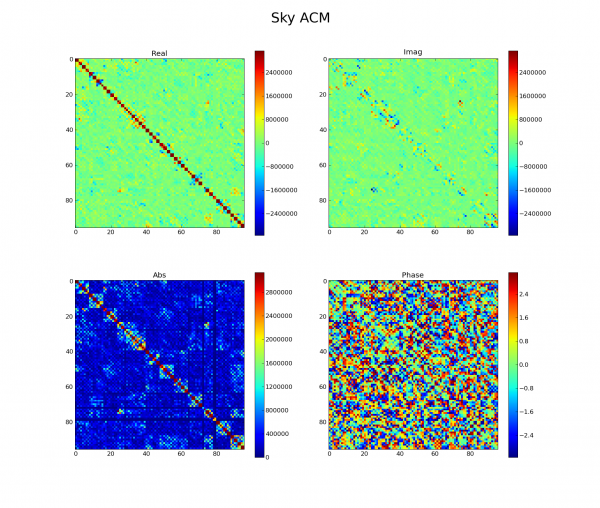
The ACMs can be inspected using the `plot_complex_image()` function. It has optional `plot_title`, `scale`, and `textsize` parameters. When `scale=True`, the _Real_ and _Abs_ plots have the same amplitude scale as the _Imag_ plot for easy comparison.

In [15]: plot_complex_image(acm_sky,'Sky visibilities sb 305')
In [16]: plot_complex_image(acm_sky,'Sky visibilities sb 305',scale=True)
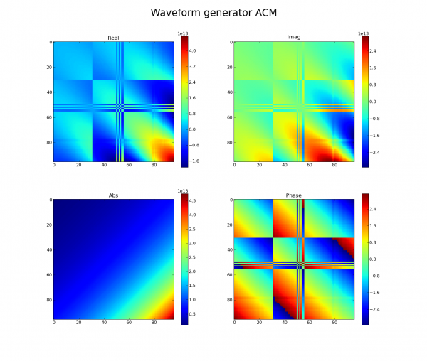
In [17]: plot_complex_image(acm_wg,'Waveform generator test sb 305')
In [18]: plot_complex_image(acm_wg,'Waveform generator test sb 305',scale=True)

In the waveform generator test the amplitude of the waveform generators increases exponentially as a function of RCU number in order to achieve a nice linear gradient on a logarithmic scale. The phases of the waveform generators span the range from 0 up to (not including) 2π.

There are a few interesting features in these plots. The first is that the _Real_ diagonal is very strong when observing the sky, whereas it does not stand out in the waveform generator test.

Why?

Let us inspect the range of values in these array correlation matrices.

In [19]: abs(acm_sky).max()
In [20]: abs(acm_sky).min()
In [21]: abs(acm_wg).max()
In [22]: abs(acm_wg).min()

There we have it.

The second is that although the amplitudes nicely show the promised exponential increase as a function of RCU number, the phases have blocks that are exactly 180 degrees out of phase. It is believed that this is caused by the fact that one cannot divide 200 million (the number of clock samples per seconds) evenly by 1024 (the length of the FFT in the polyphase filter), hence the remainder of the first second is processed in the second second, yielding a different number of samples per subband in the even seconds as compared to the odd seconds. It is believed that the n x 180 degree phase (actually a slope as a function of subband number) is due to the waveform generators starting up with a different phase in the even and odd seconds, and the fact that we cannot program all waveform generators at CS010 within one second. This claim, however, has not yet been verified. If true, the n x 180 degree phase shift should not occur when we take care to start the waveform generators all in even (or odd) seconds.

We can run some basic sanity checks on the ACMs. For one thing they should be Hermitian:

In [23]: plot_complex_image(acm_sky - transpose(conjugate(acm_sky)),
                            'Sky visibilities sb 305')
In [24]: plot_complex_image(acm_wg - transpose(conjugate(acm_wg)),
                            'Waveform generator test sb 305')

Right. We should investigate this a bit further. It appears to be a constant offset, independent of the input power.

Is that correct?

If so, is it some special value?

Let us find out.

In [25]: h = acm_wg-transpose(conjugate(acm_wg))
In [26]: h[h != 0.0]
In [27]: unique(h[h != 0.0])

What is so special about this value?

In order to track down the cause, it would be nice to see precisely when the error occurs. We can collect data from the entire frequency scan for a couple of RCUs and plot their powers as a function of subband. The functions `foreach_acm_in()` and `vis()` are very useful in this respect. The value that is plotted in input 26, for example, reads as:

   "for each ACM in directory ...., retrieve visibility 0,0"

One can pass `foreach_acm_in()` any function that operates on a 2D ACM, such as `is_hermitian()`, which is also defined below. First we plot a couple of relevant spectra.

In [25]: clf()
 
In [26]: semilogy(foreach_acm_in('array-correlation-matrices/20081204-freq-scan', vis(0,0)), label='sky rcu 0')
In [27]: semilogy(foreach_acm_in('array-correlation-matrices/20081204-freq-scan-wg', vis(0,0)), label='wg rcu 0')
In [28]: semilogy(foreach_acm_in('array-correlation-matrices/20081204-freq-scan-wg', vis(48,48)), label='wg rcu 48')
In [29]: semilogy(foreach_acm_in('array-correlation-matrices/20081204-freq-scan-wg', vis(94,94)), label='wg rcu 94')
In [30]: legend()

Then it is time to test for hermitianness in a more automatic way. We define the Python function `is_hermitian()`.

In [31]: unique((acm_sky-transpose(conjugate(acm_sky))) ==0.0)
Out[31]: array([ True], dtype=bool)
 
In [32]: unique((acm_wg-transpose(conjugate(acm_wg))) ==0.0)
Out[32]: array([False,  True], dtype=bool)
 
In [33]: def is_hermitian(matrix):
return len(unique((matrix - transpose(conjugate(matrix)))== 0.0))==1
 
In [34]: is_hermitian(acm_wg)
Out[34]: False
 
In [35]: is_hermitian(acm_sky)
Out[35]: True

Good. Now we collect data on which frequency channels are affected in the waveform generator test, and in the sky visibilities.

In [36]: sky_hermitian = foreach_acm_in('array-correlation-matrices/20081204-freq-scan', is_hermitian)
In [37]: wg_hermitian = foreach_acm_in('array-correlation-matrices/20081204-freq-scan-wg', is_hermitian)
In [38]: semilogy((sky_hermitian == False)*3e12,label='sky not hermitian')
In [39]: semilogy((wg_hermitian == False)*2e13,label='wg not hermitian')
In [40]: legend()

(note: you may have to issue a clf() command before plotting to clear the plotting window and see changes.) Apparently the error occurs when the total powers are larger than some minimum threshold value. Adventurous types may try to find out which:

In [41]: log2(min(foreach_acm_in('array-correlation-matrices/20081204-freq-scan',
lambda acm: median(diagonal(acm)))[sky_hermitian==False]))

Why?

We will continue now with analysing `acmcube`. As you may remember, this cube contains 60 second integrations for a total duration of approximately 24 hours. The function `timeseries()` can be used to retrieve the visibility of a certain RCU pair as a function of time, e.g. the XX and YY auto correlations:

In [42]: clf()
In [43]: plot(timeseries(acmcube,10,10).real,label='XX')
In [44]: plot(timeseries(acmcube,11,11).real, label='YY')
In [45]: legend()

As you can readily see, the total power peaks first in the XX correlation, followed by the YY correlation after a couple of hours.

Why?

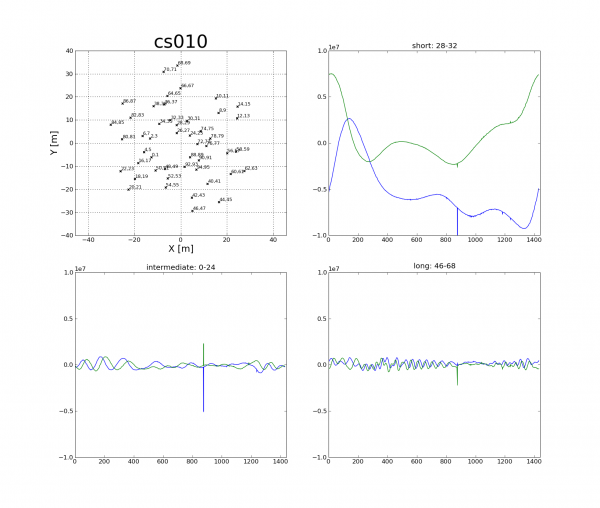
It is instructive to see the behaviour of the sky visibilities as a function of time for a number of different baselines. To that end we will build up a 2×2 panel of graphs.

In [46]: clf()
In [47]: subplot(221)
In [48]: station_map(cs010)
 
In [49]: subplot(222)
In [50]: title('short: 28-32')
In [51]: plot(timeseries(acmcube,28,32).real)
In [52]: plot(timeseries(acmcube,28,32).imag)
In [53]: axis([0,1440,-1e7,1e7])
 
In [54]: subplot(223)
In [55]: title('intermediate: 0-24')
In [56]: plot(timeseries(acmcube,0,24).real)
In [57]: plot(timeseries(acmcube,0,24).imag)
In [58]: axis([0,1440,-1e7,1e7])
 
In [59]: subplot(224)
In [60]: title('long: 46-68')
In [61]: plot(timeseries(acmcube,46,68).real)
In [62]: plot(timeseries(acmcube,46,68).imag)
In [63]: axis([0,1440,-1e7,1e7])

Fortunately the fringe frequency increases with baseline length. Furthermore, as expected, the shortest baseline picks up a lot more power than the others. This is mainly due to the large scale diffuse Galactic emission, which is not picked up at baselines beyond 4–6 wavelengths. It is clear that one needs intra-station baselines in order to properly map the diffuse Galactic foreground.

A final sanity check on the data is to plot _all_ auto correlations in the acmcube as a function of time:

In [64]: plot_autocorrelations(acmcube)

Which signal paths are flaky?

Which rcus are wired the wrong way around?

What is, in your opinion, the most striking property of the flaky signal paths?

In [65]: plot_complex_image(acm_sky, plot_title="Sky ACM", scale=True)

In [12]: plot_complex_image(acm_wg, plot_title="Waveform generator ACM")

In [46]: clf()
In [47]: subplot(221)
In [48]: station_map(cs010)
 
In [49]: subplot(222)
In [50]: title('short: 28-32')
In [51]: plot(timeseries(acmcube,28,32).real)
In [52]: plot(timeseries(acmcube,28,32).imag)
In [53]: axis([0,1440,-1e7,1e7])
 
In [54]: subplot(223)
In [55]: title('intermediate: 0-24')
In [56]: plot(timeseries(acmcube,0,24).real)
In [57]: plot(timeseries(acmcube,0,24).imag)
In [58]: axis([0,1440,-1e7,1e7])
 
In [59]: subplot(224)
In [60]: title('long: 46-68')
In [61]: plot(timeseries(acmcube,46,68).real)
In [62]: plot(timeseries(acmcube,46,68).imag)
In [63]: axis([0,1440,-1e7,1e7])

← Data Processing School