The Common Astronomy Software Applications (CASA) package is a set of C++ tools bundled together under an iPython interface as a set of data reduction tasks. CASA is being developed by a collaboration led by NRAO with the primary goal of supporting the data post-processing needs of the next generation of radio astronomical telescopes such as the ALMA and EVLA projects. This Exercise aims to demonstrate the use of CASA tasks to inspect LOFAR data.

• Working CASA installation
• Knowledge of Python

The goal of this exercise is to be able to use CASA to find out basic information about a dataset, browse the MS Tables using the CASA table browser interface, and make simple plots, such as:

• Antenna locations
• uv-coverage
• Amplitude vs uv-distance for a given baseline

• instructions.txt contains a listing of commands to be typed or cut/pasted into the CASA prompt, and explanation of what to do and what to expect at each step

• The outputs directory contains examples of output listings from the CASA logger and outputs plots from the plotting exercises

• README contains links to further documentation about CASA

First of all, start up CASA

$ /app/Casa/x86_64/bin/casapy

Then, from the CASA prompt, summarize the files in the working directory.

CASA <3>: ls
casapy.log  instructions.txt  ipython.log  outputs/  README

You should find a CS1 measurement set in this directory: L4086_sSB10.MS. Set the variable msfile to the MS name:

CASA <4>: msfile='L4086_sSB10.MS'

Now use the task listobs to print a set of summary information about the MS to the logger. Look at the logger, and check the number of antennas, observation date, central frequency, etc.

CASA <8>: default(listobs)
CASA <9>: vis=msfile
CASA <10>: inp listobs
---------> inp(listobs)
#  listobs :: List data set summary in the logger
vis                 = 'L4086_sSB10.MS' #  Name of input visibility file (MS)
verbose             =       True        
async               =      False        #  If true the taskname must be started
                                        #   using listobs(...)
CASA <11>: listobs()

Now, use the table browser to inspect the structure of the MS.

CASA <12>: default(browsetable)
CASA <13>: tablename=
CASA <14>: browsetable
---------> browsetable()

This will bring up the table browser. Examine the different subtables listed in the table keywords tab on the left hand side. Inspect the available columns. We won't do anything with them here, but data can be extracted, read into Python arrays and manipulated if necessary.

Finally, we will make a set of diagnostic plots using the task plotxy

CASA <20>: default(plotxy)
CASA <21>: vis = msfile                        
CASA <22>: antenna=''
CASA <23>: xaxis='x'
CASA <24>: go
---------> go()
Executing:  plotxy()
INFO2 Number of points being plotted : 24
Total process time 3.46 sec.
Total wall clock time 3.63 sec.

This plots up the station locations. Ignore the warning messages; LOFAR is not included in the CASA repository yet. Example output is shown in outputs/antenna_locations.pdf

Next, plot up the uv-coverage. CASA has saved the previous inputs to plotxy as plotxy.last in the working directory. Using tget will recall the last set of inputs (reminiscent of AIPS for any banana addicts out there…)

CASA <26>: tget(plotxy)
Restored parameters from file plotxy.last
CASA <27>: xaxis='u'
CASA <28>: yaxis='v'
CASA <29>: go
---------> go()
Executing:  plotxy()
INFO2 Number of points being plotted : 6079200
Total process time 54.57 sec.
Total wall clock time 54.79 sec.

It may take a while, but be patient; it is plotting 6 million points. You'll notice that the uv-coverage is pretty good. Sample output can be found at outputs/uv_coverage.pdf.

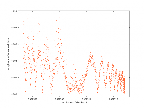
Finally, plot up amplitude against uv-distance for a single baseline. Select out a particular time range, and only the XX correlations:

CASA <33>: tget(plotxy)
Restored parameters from file plotxy.last
CASA <34>: xaxis = 'uvdist'
CASA <35>: yaxis = 'amp'
CASA <36>: datacolumn = 'data'
CASA <37>: selectdata=T
CASA <38>: correlation = 'XX'
CASA <39>: width = '1' # average all channels
CASA <40>: spw='0:1'
CASA <41>: timerange='2007/10/20/12:00:00~2007/10/20/21:00:00'
CASA <42>: antenna='1&12'
CASA <43>: go
---------> go()
Executing:  plotxy()
INFO2 Number of points being plotted : 1073
Total process time 10.18 sec.
Total wall clock time 10.47 sec.

Bad data can be flagged from the plot window. See Exercise 61 for details.

An example of the last plot produced (Amplitude vs uv-distance) is: