Continuum
Image validation
The continuum images were individually validated for every beam. In order to do this, a set of metrics was defined which inform on different aspects of image quality. The starting point of the validation are the residual images obtained after cleaning the continuum images. The validation aims at checking to what extent these images only contain Gaussian noise. The premise being that any significant deviation from this indicates issues with the calibration and/or the reduction of the data.
The following parameters were derived for each residual image.
- σin: Noise in inner half degree of the image, determined in a robust way from the residual image using the median of the absolute values.
- σout Noise at the edge of the residual image, more than a degree from the centre determined in a robust way from the residual image using the median of the absolute values. This value is taken as a reasonable measure of the expected noise.
- R=σin/σout: A measure of the strength of artifacts left in the centre of the residual image.
- Ex-2: Area, in units of beam area, with values below 2 σout in the inner 0.5 degree of the residual image, in excess of what expected from a purely Gaussian distribution. For perfect noise Ex-2 = 0.
- MaxNeg: the level, in units of σout, at which the area covered by pixels with values below this level is 10 beams. The expected value is -3.2. More negative values indicate significant negative calibration residuals.
Note that we did not use the equivalents of the parameters Ex-2 and MaxNeg based on positive deviations from Gaussianity (Ex+2 and MaxPos). This is because many residual images have weak, positive residuals due to insufficient cleaning which would then dominate the validation.
Visual examination of a large set of images was undertaken to define the numerical criteria that would catch significant image artifacts, as used above. The main types of image artifacts due to errors in the selfcalibration as well as strong direction-dependent errors for which the calibration pipeline did not attempt to correct. The criteria were set so that the large majority of images which were visually assessed as good would pass while only a small fraction of images that were visually assessed as bad would be classified as good.
The final criteria used to reject images are:
- R > 1.225. This criterion catches stripes due to errors in the amplitude calibration.
- R > 1.15, MaxNeg < -4.5 and Ex-2>400. This criterion catches general image artifacts and deviations from Gaussianity in the residual image.
Two additional criteria were set based on survey specifications:
- σin or σout > 60 microJy/beam. In this case the noise of the image does not meet the minimum requirement to be considered survey quality and valid.
- The minor axis of the restoring beam is > 15 arcsec. This occurs when both dishes RTC and RTD are missing from an observation. In this case, the required angular resolution of the survey is not met.
Flux scale & astrometry
For checking the consistency of the flux scale two beams of an observation of a field in the Perseus-Pisces region centered on RA(J2000) = 01h55m and Dec(J2000) = 33d56’ which was observed ten times between September 2019 and January 2020 were examined. The automatic source finder PyBDSF (also used in the Apercal pipeline) was used to find and determine source fluxes, positions and sizes and compared these from observation to observation. We restricted the comparison to sources that are less than 35” in size and have fluxes above 3 mJy (100 times the typical rms noise) and agree in position to within 3 arcsecs to ensure that the sources used for comparison are indeed identical and have been included in the clean masks.
The overall consistency is very good with a mean of 1.014 and an rms of 4% . If one excludes the two most discrepant observations (ObsID 191207035 and 191227014) the rms decreases to 2%. Table 1 provides the flux ratio of 10 observations relative to the last observation made on 06.01.2020 (ObsID 200106010)
Table 1
| ObsID | median Flux Ratio |
| 190919049 | 0.9982 |
| 191207035 | 0.9311 |
| 191223022 | 1.0041 |
| 191225015 | 1.0116 |
| 191227014 | 1.1069 |
| 191229014 | 1.0185 |
| 191231013 | 1.0062 |
| 200102012 | 1.0446 |
| 200104011 | 1.0222 |
| 200106010 | 1.0000 |
An example of two observations (ObsID 200106010 and 190909049, observed at 06.01.2020 and 09.09.2019 respectively) compared to one another is shown in Figure 1. Plotted is the relative difference in flux versus the flux in the 06.01.2020 observation.

To assess the agreement with the NVSS we made mosaics of the full field of view (40 beams) of all observations using the measured shapes of the 40 beams. The reason for using mosaics rather than individual beams was to have a large enough number of sources for the comparison as in an individual beam there usually are only of order a dozen that are bright enough. The mosaicing routine takes into account shapes of the beams made with the phased array feeds as determined from drift scans across Cygnus A (see the section on Primary beam response: Drift scan method) and corrects for the presence of correlated noise in adjacent beams. The mosaics were made with a resolution of 28″ x 28″. We ran PyBDSF on the mosaics to produce a source catalog and compared sources in this catalogue with the sources in the NVSS source catalog extracted from VizieR. For the comparison we restricted ourselves to sources that agree in position to within 4″, are less than 28.5″ in size and stronger than 3 mJy in the Apertif mosaic.
Table 2 captures the comparison of the individual mosaics with the NVSS. For each ObsID the median flux ratio NVSS / Apertif is given. On average the Apertif flux scale is 3% above the NVSS flux scale for these mosaics with an rms of 4%. If the two most discrepant ObsIDs are omitted (191207035 and 191227014) the rms reduces to 2%. Figure 2 illustrates the agreement between the Apertif and NVSS flux scale for ObsID 200102012. Since the observing frequency of the mosaic is 1360 MHz as opposed to the 1400 MHz of NVSS ~2% of the flux difference can be accounted for by spectral index effects (assuming an average spectral index of -0.7) which were not taken into account.
Table 2
| ObsID | median Flux Ratio |
| 190919049 | 0.943 |
| 191207035 | 0.894 |
| 191223022 | 0.962 |
| 191225015 | 0.969 |
| 191227014 | 1.083 |
| 191229014 | 0.980 |
| 191231013 | 0.974 |
| 200102012 | 1.004 |
| 200104011 | 0.976 |
| 200106010 | 0.964 |

This is described in “Characterization of the primary beams” and yields a current estimate of the flux scale of Apertif as compared to NVSS. From this comparison the Apertif fluxes are on average 9% higher than those of NVSS, accounting for a nominal spectral index of the sources of -0.7.
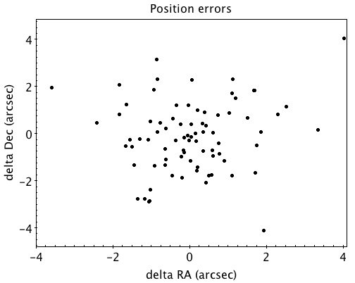
Since we had to match sources in Apertif and NVSS for the source comparison we also obtained information on the agreement between the Apertif and NVSS astrometry. Figure 3 shows the positional differences for sources in the mosaic of ObsID 200102012 and the NVSS catalogue. The agreement is very good with mean offsets of 0.05 +/- 0.2 arcsec in RA and -0.05 +/- 0.2 arcsec in Dec.
SEE ALSO: